sparklyr-R语言访问Spark的另外一种方法
Spark自带了R语言的支持-SparkR,前面我也介绍了最简便的SparkR安装方法,这里我们换个方式,使用Rstudio提供的接口,sparklyr。
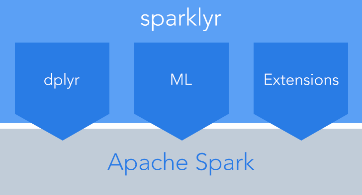
- 提供了完整的 dplyr后台实现
- 方便与Spark MLlib or H2O Sparkling Water整合
- 方便基于SPARK API编写自己的扩展
安装(记得安装Java虚拟机),
devtools::install_github("rstudio/sparklyr")
#install.packages("sparklyr")
#以上两种方法都可以

library(sparklyr)

#选择spark和hadoop的版本
spark_install(version = "2.0.1",hadoop_version = "2.7")
连接Spark
library(sparklyr)
sc <- spark_connect(master = "local")
读取数据
#install.packages(c("nycflights13", "Lahman"))
library(dplyr)
iris_tbl <- copy_to(sc, iris)
flights_tbl <- copy_to(sc, nycflights13::flights, "flights")
batting_tbl <- copy_to(sc, Lahman::Batting, "batting")
列出所有的表
>src_tbls(sc)
[1] "batting" "flights" "iris"
使用dplyr
# filter by departure delay and print the first few records
>flights_tbl %>% filter(dep_delay == 2)

## Source:   query [?? x 19]
## Database: spark connection master=local[8] app=sparklyr local=TRUE
##
##     year month   day dep_time sched_dep_time dep_delay arr_time
##    <int> <int> <int>    <int>          <int>     <dbl>    <int>
## 1   2013     1     1      517            515         2      830
## 2   2013     1     1      542            540         2      923
## 3   2013     1     1      702            700         2     1058
## 4   2013     1     1      715            713         2      911
## 5   2013     1     1      752            750         2     1025
## 6   2013     1     1      917            915         2     1206
## 7   2013     1     1      932            930         2     1219
## 8   2013     1     1     1028           1026         2     1350
## 9   2013     1     1     1042           1040         2     1325
## 10  2013     1     1     1231           1229         2     1523
## # ... with more rows, and 12 more variables: sched_arr_time <int>,
## #   arr_delay <dbl>, carrier <chr>, flight <int>, tailnum <chr>,
## #   origin <chr>, dest <chr>, air_time <dbl>, distance <dbl>, hour <dbl>,
## #   minute <dbl>, time_hour <dbl>
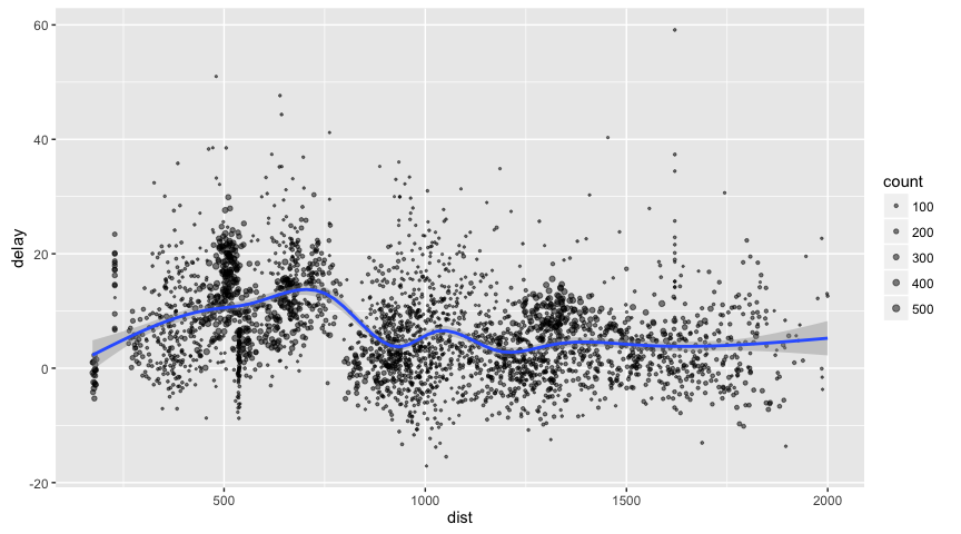
画图
delay <- flights_tbl %>%
  group_by(tailnum) %>%
  summarise(count = n(), dist = mean(distance), delay = mean(arr_delay)) %>%
  filter(count > 20, dist < 2000, !is.na(delay)) %>%
  collect

# plot delays
library(ggplot2)
ggplot(delay, aes(dist, delay)) +
  geom_point(aes(size = count), alpha = 1/2) +
  geom_smooth() +
  scale_size_area(max_size = 2)
开窗函数Window Function
batting_tbl %>%
  select(playerID, yearID, teamID, G, AB:H) %>%
  arrange(playerID, yearID, teamID) %>%
  group_by(playerID) %>%
  filter(min_rank(desc(H)) <= 2 & H > 0)

## Source:   query [?? x 7]
## Database: spark connection master=local[8] app=sparklyr local=TRUE
## Groups: playerID
##
##     playerID yearID teamID     G    AB     R     H
##        <chr>  <int>  <chr> <int> <int> <int> <int>
## 1  abbotpa01   2000    SEA    35     5     1     2
## 2  abbotpa01   2004    PHI    10    11     1     2
## 3  abnersh01   1992    CHA    97   208    21    58
## 4  abnersh01   1990    SDN    91   184    17    45
## 5  abreujo02   2015    CHA   154   613    88   178
## 6  abreujo02   2014    CHA   145   556    80   176
## 7  acevejo01   2001    CIN    18    34     1     4
## 8  acevejo01   2004    CIN    39    43     0     2
## 9  adamsbe01   1919    PHI    78   232    14    54
## 10 adamsbe01   1918    PHI    84   227    10    40
## # ... with more rows
使用SQL
library(DBI)
iris_preview <- dbGetQuery(sc, "SELECT * FROM iris LIMIT 10")
iris_preview

##    Sepal_Length Sepal_Width Petal_Length Petal_Width Species
## 1           5.1         3.5          1.4         0.2  setosa
## 2           4.9         3.0          1.4         0.2  setosa
## 3           4.7         3.2          1.3         0.2  setosa
## 4           4.6         3.1          1.5         0.2  setosa
## 5           5.0         3.6          1.4         0.2  setosa
## 6           5.4         3.9          1.7         0.4  setosa
## 7           4.6         3.4          1.4         0.3  setosa
## 8           5.0         3.4          1.5         0.2  setosa
## 9           4.4         2.9          1.4         0.2  setosa
## 10          4.9         3.1          1.5         0.1  setosa
机器学习
# copy mtcars into spark
mtcars_tbl <- copy_to(sc, mtcars)

# transform our data set, and then partition into 'training', 'test'
partitions <- mtcars_tbl %>%
  filter(hp >= 100) %>%
  mutate(cyl8 = cyl == 8) %>%
  sdf_partition(training = 0.5, test = 0.5, seed = 1099)

# fit a linear model to the training dataset
fit <- partitions$training %>%
  ml_linear_regression(response = "mpg", features = c("wt", "cyl"))

## * No rows dropped by 'na.omit' call
fit
## Call: ml_linear_regression(., response = "mpg", features = c("wt", "cyl"))
##
## Coefficients:
## (Intercept)          wt         cyl
##   37.066699   -2.309504   -1.639546
summary(fit)
## Call: ml_linear_regression(., response = "mpg", features = c("wt", "cyl"))
##
## Deviance Residuals::
##     Min      1Q  Median      3Q     Max
## -2.6881 -1.0507 -0.4420  0.4757  3.3858
##
## Coefficients:
##             Estimate Std. Error t value  Pr(>|t|)
## (Intercept) 37.06670    2.76494 13.4059 2.981e-07 ***
## wt          -2.30950    0.84748 -2.7252   0.02341 *
## cyl         -1.63955    0.58635 -2.7962   0.02084 *
## ---
## Signif. codes:  0 '***' 0.001 '**' 0.01 '*' 0.05 '.' 0.1 ' ' 1
##
## R-Squared: 0.8665
## Root Mean Squared Error: 1.799
读写数据
temp_csv <- tempfile(fileext = ".csv")
temp_parquet <- tempfile(fileext = ".parquet")
temp_json <- tempfile(fileext = ".json")

spark_write_csv(iris_tbl, temp_csv)
iris_csv_tbl <- spark_read_csv(sc, "iris_csv", temp_csv)

spark_write_parquet(iris_tbl, temp_parquet)
iris_parquet_tbl <- spark_read_parquet(sc, "iris_parquet", temp_parquet)

spark_write_csv(iris_tbl, temp_json)
iris_json_tbl <- spark_read_csv(sc, "iris_json", temp_json)

src_tbls(sc)
## [1] "batting"      "flights"      "iris"         "iris_csv"
## [5] "iris_json"    "iris_parquet" "mtcars"
编写扩展
# write a CSV
tempfile <- tempfile(fileext = ".csv")
write.csv(nycflights13::flights, tempfile, row.names = FALSE, na = "")

# define an R interface to Spark line counting
count_lines <- function(sc, path) {
  spark_context(sc) %>%
    invoke("textFile", path, 1L) %>%
      invoke("count")
}

# call spark to count the lines of the CSV
count_lines(sc, tempfile)
## [1] 336777
dplyr Utilities
tbl_cache(sc, "batting") #把表载入内存
tbl_uncache(sc, "batting") #把表从内存中卸载
连接Utilities
spark_web(sc) #Spark web console
spark_log(sc, n = 10) #输出日志
关闭与Spark的连接
spark_disconnect(sc)